[本文来自：www.11jj.com]

YouTube网红小哥Siraj Raval系列视频又和大家见面啦！今天要讲的是加密货币价格预测，包含大量代码，还用一个视频详解具体步骤，不信你看了还学不会！

点击观看详解视频

时长22分钟

有中文字幕

▼

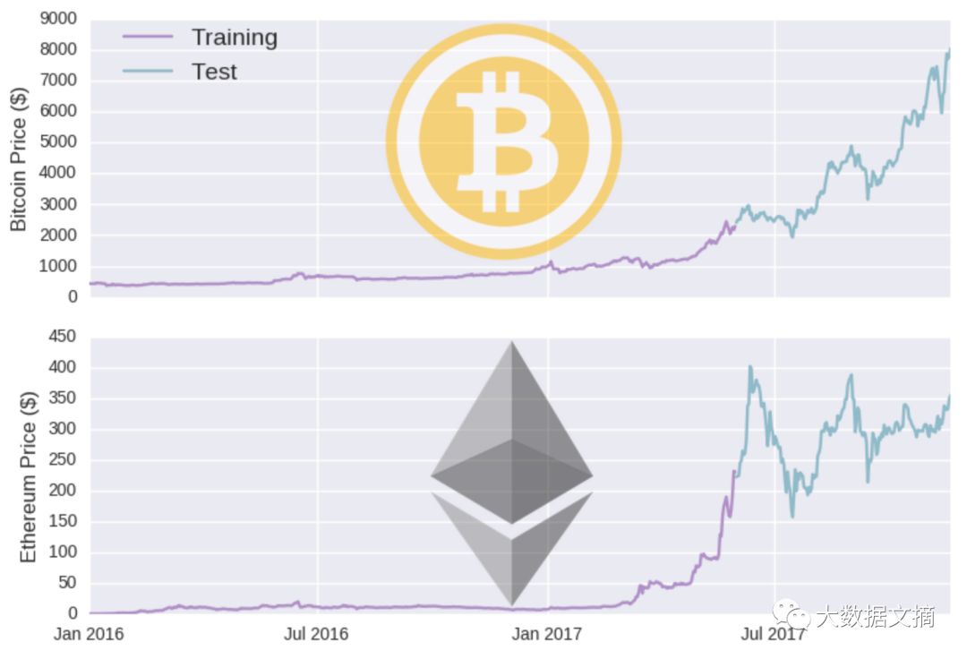
预测加密货币价格其实很简单，用Python+Keras，再来一个循环神经网络（确切说是双向LSTM），只需要9步就可以了！..以太坊价格预测都不在话下。

这9个步骤是：

数据处理

建模

训练模型

测试模型

分析价格变化

分析价格百分比变化

比较预测值和实际数据

计算模型评估指标

结合在一起：可视化

数据处理

导入Keras、Scikit learn的metrics、numpy、pandas、matplotlib这些我们需要的库。

## Keras for deep learning
from keras.layers.core import Dense, Activation, Dropout
from keras.layers.recurrent import LSTM
from keras.layers import Bidirectional
from keras.models import Sequential

## Scikit learn for mapping metrics
from sklearn.metrics import mean_squared_error

#for logging
import time

##matrix math
import numpy as np
import math

##plotting
import matplotlib.pyplot as plt

##data processing
import pandas as pd

首先，要对数据进行归一化处理。关于数据处理的原则，有张大图，大家可以在大数据文摘公众号后台对话框内回复“加密货币”查看高清图。

def load_data(filename, sequence_length):
   """
   Loads the bitcoin data
   
   Arguments:
   filename -- A string that represents where the .csv file can be located
   sequence_length -- An integer of how many days should be looked at in a row
   
   Returns:
   X_train -- A tensor of shape (2400, 49, 35) that will be inputed into the model to train it
   Y_train -- A tensor of shape (2400,) that will be inputed into the model to train it
   X_test -- A tensor of shape (267, 49, 35) that will be used to test the model"s proficiency
   Y_test -- A tensor of shape (267,) that will be used to check the model"s predictions
   Y_daybefore -- A tensor of shape (267,) that represents the price of bitcoin the day before each Y_test value
   unnormalized_bases -- A tensor of shape (267,) that will be used to get the true prices from the normalized ones
   window_size -- An integer that represents how many days of X values the model can look at at once
   """
   #Read the data file
   raw_data = pd.read_csv(filename, dtype = float).values
   
   #Change all zeros to the number before the zero occurs
   for x in range(0, raw_data.shape[0]):
       for y in range(0, raw_data.shape[1]):
           if(raw_data[x][y] == 0):
               raw_data[x][y] = raw_data[x-1][y]
   
   #Convert the file to a list
   data = raw_data.tolist()
   
   #Convert the data to a 3D array (a x b x c)
   #Where a is the number of days, b is the window size, and c is the number of features in the data file
   result = []
   for index in range(len(data) - sequence_length):
       result.append(data[index: index + sequence_length])
   
   #Normalizing data by going through each window
   #Every value in the window is divided by the first value in the window, and then 1 is subtracted
   d0 = np.array(result)
   dr = np.zeros_like(d0)
   dr[:,1:,:] = d0[:,1:,:] / d0[:,0:1,:] - 1
   
   #Keeping the unnormalized prices for Y_test
   #Useful when graphing bitcoin price over time later
   start = 2400
   end = int(dr.shape[0] + 1)
   unnormalized_bases = d0[start:end,0:1,20]
   
   #Splitting data set into training (First 90% of data points) and testing data (last 10% of data points)
   split_line = round(0.9 * dr.shape[0])
   training_data = dr[:int(split_line), :]
   
   #Shuffle the data
   np.random.shuffle(training_data)
   
   #Training Data
   X_train = training_data[:, :-1]
   Y_train = training_data[:, -1]
   Y_train = Y_train[:, 20]
   
   #Testing data
   X_test = dr[int(split_line):, :-1]
   Y_test = dr[int(split_line):, 49, :]
   Y_test = Y_test[:, 20]

   #Get the day before Y_test"s price
   Y_daybefore = dr[int(split_line):, 48, :]
   Y_daybefore = Y_daybefore[:, 20]
   
   #Get window size and sequence length
   sequence_length = sequence_length
   window_size = sequence_length - 1 #because the last value is reserved as the y value
   
   return X_train, Y_train, X_test, Y_test, Y_daybefore, unnormalized_bases, window_size

建模

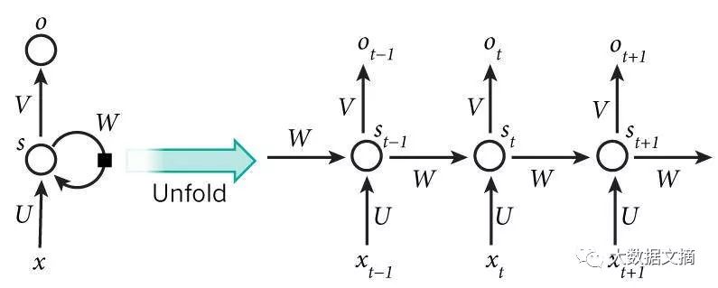
我们用到的是一个3层RNN，dropout率20%。

双向RNN基于这样的想法：时间t的输出不仅依赖于序列中的前一个元素，而且还可以取决于未来的元素。比如，要预测一个序列中缺失的单词，需要查看左侧和右侧的上下文。双向RNN是两个堆叠在一起的RNN，根据两个RNN的隐藏状态计算输出。

举个例子，这句话里缺失的单词gym要查看上下文才能知道（文摘菌：everyday?）：

I go to the (  ) everyday to get fit.

def initialize_model(window_size, dropout_value, activation_function, loss_function, optimizer):
   """
   Initializes and creates the model to be used
   
   Arguments:
   window_size -- An integer that represents how many days of X_values the model can look at at once
   dropout_value -- A decimal representing how much dropout should be incorporated at each level, in this case 0.2
   activation_function -- A string to define the activation_function, in this case it is linear
   loss_function -- A string to define the loss function to be used, in the case it is mean squared error
   optimizer -- A string to define the optimizer to be used, in the case it is adam
   
   Returns:
   model -- A 3 layer RNN with 100*dropout_value dropout in each layer that uses activation_function as its activation
            function, loss_function as its loss function, and optimizer as its optimizer
   """
   #Create a Sequential model using Keras
   model = Sequential()

   #First recurrent layer with dropout
   model.add(Bidirectional(LSTM(window_size, return_sequences=True), input_shape=(window_size, X_train.shape[-1]),))
   model.add(Dropout(dropout_value))

   #Second recurrent layer with dropout
   model.add(Bidirectional(LSTM((window_size*2), return_sequences=True)))
   model.add(Dropout(dropout_value))

   #Third recurrent layer
   model.add(Bidirectional(LSTM(window_size, return_sequences=False)))

   #Output layer (returns the predicted value)
   model.add(Dense(units=1))
   
   #Set activation function
   model.add(Activation(activation_function))

   #Set loss function and optimizer
   model.compile(loss=loss_function, optimizer=optimizer)
   
   return model

训练模型

这里取batch size = 1024，epoch times = 100。我们需要最小化均方误差MSE。

def fit_model(model, X_train, Y_train, batch_num, num_epoch, val_split):
   """
   Fits the model to the training data
   
   Arguments:
   model -- The previously initalized 3 layer Recurrent Neural Network
   X_train -- A tensor of shape (2400, 49, 35) that represents the x values of the training data
   Y_train -- A tensor of shape (2400,) that represents the y values of the training data
   batch_num -- An integer representing the batch size to be used, in this case 1024
   num_epoch -- An integer defining the number of epochs to be run, in this case 100
   val_split -- A decimal representing the proportion of training data to be used as validation data
   
   Returns:
   model -- The 3 layer Recurrent Neural Network that has been fitted to the training data
   training_time -- An integer representing the amount of time (in seconds) that the model was training
   """
   #Record the time the model starts training
   start = time.time()

   #Train the model on X_train and Y_train
   model.fit(X_train, Y_train, batch_size= batch_num, nb_epoch=num_epoch, validation_split= val_split)

   #Get the time it took to train the model (in seconds)
   training_time = int(math.floor(time.time() - start))
   return model, training_time

测试模型

def test_model(model, X_test, Y_test, unnormalized_bases):
   """
   Test the model on the testing data
   
   Arguments:
   model -- The previously fitted 3 layer Recurrent Neural Network
   X_test -- A tensor of shape (267, 49, 35) that represents the x values of the testing data
   Y_test -- A tensor of shape (267,) that represents the y values of the testing data
   unnormalized_bases -- A tensor of shape (267,) that can be used to get unnormalized data points
   
   Returns:
   y_predict -- A tensor of shape (267,) that represnts the normalized values that the model predicts based on X_test
   real_y_test -- A tensor of shape (267,) that represents the actual prices of bitcoin throughout the testing period
   real_y_predict -- A tensor of shape (267,) that represents the model"s predicted prices of bitcoin
   fig -- A branch of the graph of the real predicted prices of bitcoin versus the real prices of bitcoin
   """
   #Test the model on X_Test
   y_predict = model.predict(X_test)

   #Create empty 2D arrays to store unnormalized values
   real_y_test = np.zeros_like(Y_test)
   real_y_predict = np.zeros_like(y_predict)

   #Fill the 2D arrays with the real value and the predicted value by reversing the normalization process
   for i in range(Y_test.shape[0]):
       y = Y_test[i]
       predict = y_predict[i]
       real_y_test[i] = (y+1)*unnormalized_bases[i]
       real_y_predict[i] = (predict+1)*unnormalized_bases[i]

   #Plot of the predicted prices versus the real prices
   fig = plt.figure(figsize=(10,5))
   ax = fig.add_subplot(111)
   ax.set_title("Bitcoin Price Over Time")
   plt.plot(real_y_predict, color = "green", label = "Predicted Price")
   plt.plot(real_y_test, color = "red", label = "Real Price")
   ax.set_ylabel("Price (USD)")
   ax.set_xlabel("Time (Days)")
   ax.legend()
   
   return y_predict, real_y_test, real_y_predict, fig

分析价格变化

def price_change(Y_daybefore, Y_test, y_predict):
   """
   Calculate the percent change between each value and the day before
   
   Arguments:
   Y_daybefore -- A tensor of shape (267,) that represents the prices of each day before each price in Y_test
   Y_test -- A tensor of shape (267,) that represents the normalized y values of the testing data
   y_predict -- A tensor of shape (267,) that represents the normalized y values of the model"s predictions
   
   Returns:
   Y_daybefore -- A tensor of shape (267, 1) that represents the prices of each day before each price in Y_test
   Y_test -- A tensor of shape (267, 1) that represents the normalized y values of the testing data
   delta_predict -- A tensor of shape (267, 1) that represents the difference between predicted and day before values
   delta_real -- A tensor of shape (267, 1) that represents the difference between real and day before values
   fig -- A plot representing percent change in bitcoin price per day,
   """
   #Reshaping Y_daybefore and Y_test
   Y_daybefore = np.reshape(Y_daybefore, (-1, 1))
   Y_test = np.reshape(Y_test, (-1, 1))

   #The difference between each predicted value and the value from the day before
   delta_predict = (y_predict - Y_daybefore) / (1+Y_daybefore)

   #The difference between each true value and the value from the day before
   delta_real = (Y_test - Y_daybefore) / (1+Y_daybefore)

   #Plotting the predicted percent change versus the real percent change
   fig = plt.figure(figsize=(10, 6))
   ax = fig.add_subplot(111)
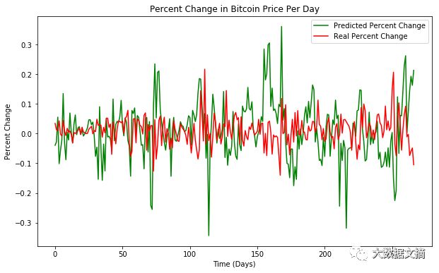
   ax.set_title("Percent Change in Bitcoin Price Per Day")
   plt.plot(delta_predict, color="green", label = "Predicted Percent Change")
   plt.plot(delta_real, color="red", label = "Real Percent Change")
   plt.ylabel("Percent Change")
   plt.xlabel("Time (Days)")
   ax.legend()
   plt.show()
   
   return Y_daybefore, Y_test, delta_predict, delta_real, fig

分析价格百分比变化

def binary_price(delta_predict, delta_real):
   """
   Converts percent change to a binary 1 or 0, where 1 is an increase and 0 is a decrease/no change
   
   Arguments:
   delta_predict -- A tensor of shape (267, 1) that represents the predicted percent change in price
   delta_real -- A tensor of shape (267, 1) that represents the real percent change in price
   
   Returns:
   delta_predict_1_0 -- A tensor of shape (267, 1) that represents the binary version of delta_predict
   delta_real_1_0 -- A tensor of shape (267, 1) that represents the binary version of delta_real
   """
   #Empty arrays where a 1 represents an increase in price and a 0 represents a decrease in price
   delta_predict_1_0 = np.empty(delta_predict.shape)
   delta_real_1_0 = np.empty(delta_real.shape)

   #If the change in price is greater than zero, store it as a 1
   #If the change in price is less than zero, store it as a 0
   for i in range(delta_predict.shape[0]):
       if delta_predict[i][0] > 0:
           delta_predict_1_0[i][0] = 1
       else:
           delta_predict_1_0[i][0] = 0
   for i in range(delta_real.shape[0]):
       if delta_real[i][0] > 0:
           delta_real_1_0[i][0] = 1
       else:
           delta_real_1_0[i][0] = 0    

   return delta_predict_1_0, delta_real_1_0

比较预测值和实际数据

def find_positives_negatives(delta_predict_1_0, delta_real_1_0):
   """
   Finding the number of false positives, false negatives, true positives, true negatives
   
   Arguments:
   delta_predict_1_0 -- A tensor of shape (267, 1) that represents the binary version of delta_predict
   delta_real_1_0 -- A tensor of shape (267, 1) that represents the binary version of delta_real
   
   Returns:
   true_pos -- An integer that represents the number of true positives achieved by the model
   false_pos -- An integer that represents the number of false positives achieved by the model
   true_neg -- An integer that represents the number of true negatives achieved by the model
   false_neg -- An integer that represents the number of false negatives achieved by the model
   """
   #Finding the number of false positive/negatives and true positives/negatives
   true_pos = 0
   false_pos = 0
   true_neg = 0
   false_neg = 0
   for i in range(delta_real_1_0.shape[0]):
       real = delta_real_1_0[i][0]
       predicted = delta_predict_1_0[i][0]
       if real == 1:
           if predicted == 1:
               true_pos += 1
           else:
               false_neg += 1
       elif real == 0:
           if predicted == 0:
               true_neg += 1
           else:
               false_pos += 1
   return true_pos, false_pos, true_neg, false_neg

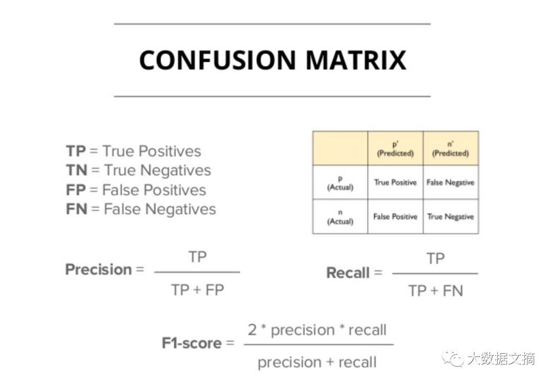
计算模型评估指标

def calculate_statistics(true_pos, false_pos, true_neg, false_neg, y_predict, Y_test):
  """
  Calculate various statistics to assess performance
 
  Arguments:
  true_pos -- An integer that represents the number of true positives achieved by the model
  false_pos -- An integer that represents the number of false positives achieved by the model
  true_neg -- An integer that represents the number of true negatives achieved by the model
  false_neg -- An integer that represents the number of false negatives achieved by the model
  Y_test -- A tensor of shape (267, 1) that represents the normalized y values of the testing data
  y_predict -- A tensor of shape (267, 1) that represents the normalized y values of the model"s predictions
 
  Returns:
  precision -- How often the model gets a true positive compared to how often it returns a positive
  recall -- How often the model gets a true positive compared to how often is hould have gotten a positive
  F1 -- The weighted average of recall and precision
  Mean Squared Error -- The average of the squares of the differences between predicted and real values
  """
  precision = float(true_pos) / (true_pos + false_pos)
  recall = float(true_pos) / (true_pos + false_neg)
  F1 = float(2 * precision * recall) / (precision + recall)
  #Get Mean Squared Error
  MSE = mean_squared_error(y_predict.flatten(), Y_test.flatten())

  return precision, recall, F1, MSE

结合在一起：可视化

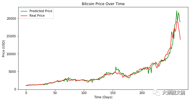
终于可以看看我们的成果啦！

首先是预测价格vs实际价格：

y_predict, real_y_test, real_y_predict, fig1 = test_model(model, X_test, Y_test, unnormalized_bases)

#Show the plot
plt.show(fig1)

然后是预测的百分比变化vs实际的百分比变化，值得注意的是，这里的预测相对实际来说波动更大，这是模型可以提高的部分：

Y_daybefore, Y_test, delta_predict, delta_real, fig2 = price_change(Y_daybefore, Y_test, y_predict)

#Show the plot
plt.show(fig2)

最终模型表现是这样的：

Precision: 0.62
Recall: 0.553571428571
F1 score: 0.584905660377
Mean Squared Error: 0.0430756924477

怎么样，看完有没有跃跃欲试呢？

代码下载地址：

http://github.com/llSourcell/ethereum_future/blob/master/A%20Deep%20Learning%20Approach%20to%20Predicting%20Cryptocurrency%20Prices.ipynb

原视频地址：

http://www.youtube.com/watch?v=G5Mx7yYdEhE

作    者 | Siraj Raval 大数据文摘经授权译制

翻    译 | 糖竹子、狗小白、邓子稷

时间轴 | 韩振峰、Barbara、菜菜Tom

监    制 | 龙牧雪

【今日机器学习概念】

Have a Great Definition

志愿者介绍

回复“志愿者”加入我们